- Compute the observed trend in the phenomenon under consideration (excluding the event itself).
- Relate the event quantitatively by physical and observational arguments to a quantity for which a model-based attribution study has been performed
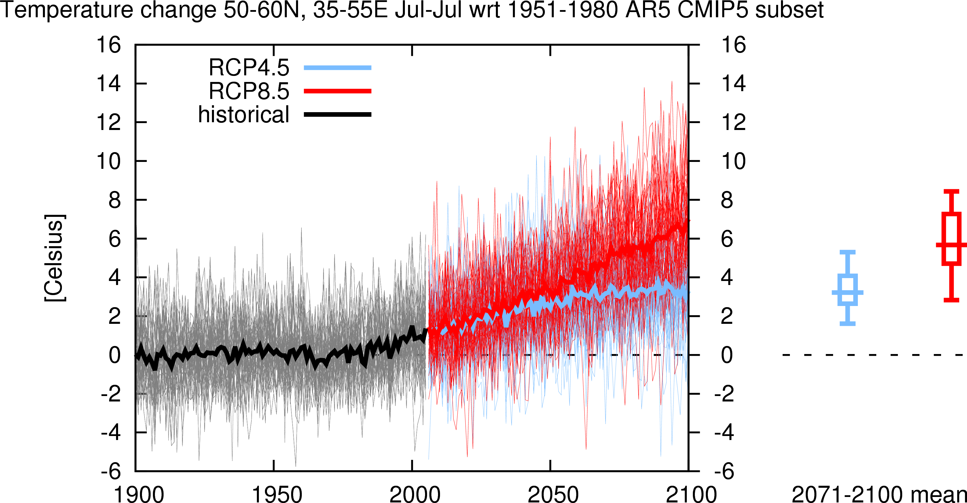
The area average 50°-60°N, 35°-55°E in the GISTEMP 1200 dataset for July is shown below.

This immediately presents a problem. The low-pass filtered temperature follows the global mean temperature well after 1950, but has very high values also in the 1930s. The decision whether to include these (Dole et al, GRL, 2011) or not (Otto et al, 2012) is a subjective one. On the basis of observed discontinuities in individual station series during the second world war we concluded that the cooling from the 1930s to the 1950s is likely an artefact caused by station changes and we started our analysis in 1950.
This series has to be analysed with a GPD fit, where we shift the distribution with the global mean temperature. There is evidence that high extremes increase faster than the mean, but we do not have enough information to take that into account in this fit. It should be investigated how this affects the result. We take a threshold of 80% and constrain the shape parameter ξ to be roughly in the interval ±0.2 to get better convergence (especially in the bootstrapped error margins). The fit gives a small ξ and the fitted line agrees well with the data points, so this is a reasonable choice. The fit results are
| Jul GISS_1200_T2m/SST_anom_35-55E_50-60N tempanomaly [Celsius] dependent on GISS global temperature | |||
|---|---|---|---|
| covariatie 1950 = | -0.11521 | ||
| covariatie 2010 = | 0.57083 | ||
| parameter | year | value | 95% CI |
| N: | 63 | ||
| Fitted to GPD distribution H(x+a') = 1 - (1+ξ*x/b')^(-1/ξ) | |||
| with a'= a+αT and b' = b | |||
| a: | 1.337 | 1.138... 3.529 | |
| b: | 0.732 | 0.192... 0.872 | |
| ξ: | -0.032 | -0.049... 0.115 | |
| α: | 1.906 | -0.518... 10.719 | |
| return period 2010 | 1950 | 2635.9 | 13.636 ... 0.31326E+09 |
| (value 4.8858 ) | 2010 | 318.17 | 2.1290 ... 24597. |
| ratio | 8.2847 | 0.22238 ... 0.43287E+07 | |
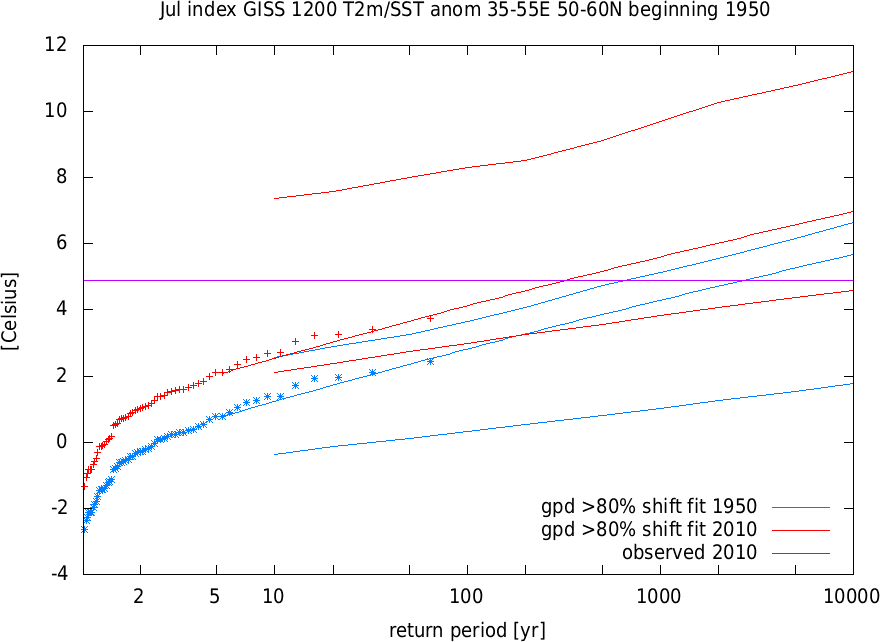
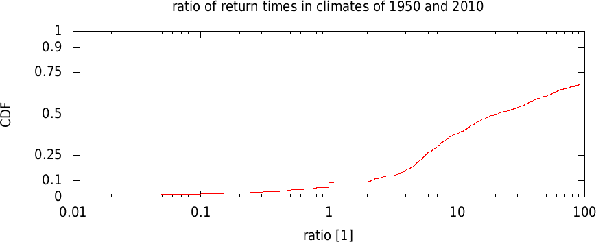
Based on the trend over 1950-2014, heat waves like his have become more likely with a p-value p<0.1: the CDF crosses 1 at around 0.07:
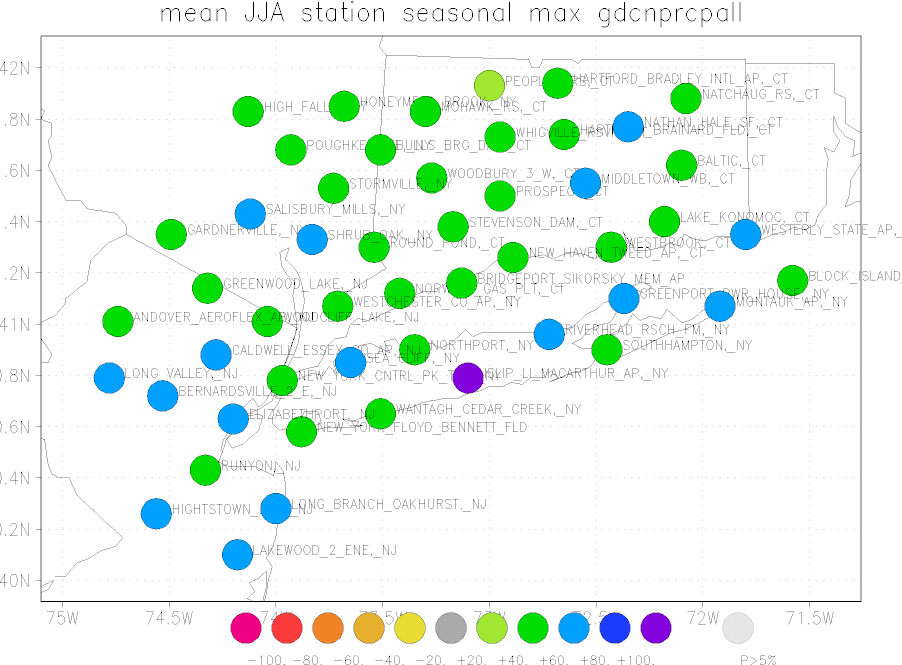
Next we have to check whether these stations are comparable in their rainfall climate. As a first check I computed the mean of the maximum precipitation in June-August. The first time this takes a while as the station data has to be converted from the GHCN-D format into the Climate Explorer format. Subsequent operations on the same data are much faster. There are no obvious structures in the map, such as more intense showers on the coast, to the south or over the city of New York. We therefore consider all these stations identically distributed.
Next we can compute extreme value statistics. For this we take summer maximum of precipitation and fit it to a GEV distribution. (NOTE: The GPD(T) routine still has issues at this moment, 4 September 2014.) We consider June-August again to exclude tropical storms and winter storms. The summer maximum can be specified in two ways: either by operating on the time series after selecting the set, or in the form 'trends in return times of extremes'. The latter offers more flexibility, but gives slightly different results at the moment, I am investigating where the differences come from. A full investigation should add the tropical storms and winter storms as well.
As a covariate I use low-pass filtered global mean temperature. Let's compare the current climate, 2014, with 1951. There are two options to include the observed extreme. The first is to wait until the data is available in the GHCN-D database. This is updated daily at NCDC, but only monthly in the Climate Explorer. Either wait until the next month or ask me to run the update by hand. The second option is to specify the value reported from another source in the form (after converting from inches to mm for the US). Finally, we scale the distribution with the global mean temperature, which is often a good choice for precipitation . (I am working on the option to fit location and scale parameters independently.) This should give output similar to the following.
| JJA gdcnprcpall max_PRCP [mm/day] dependent on GISS global temperature | |||
|---|---|---|---|
| covariatie 1951 = | -0.85208E-01 | ||
| covariatie 2014 = | 0.60375 | ||
| parameter | year | value | 95% CI |
| N: | 1985 | ||
| Fitted to GEV distribution P(x) = exp(-(1+ξ(x-a')/b')^(-1/ξ)) | |||
| with a' = a exp(αT/a) and b' = b exp(αT/a) | |||
| a': | 1951 | 59.735 | 58.881... 61.108 |
| b': | 1951 | 18.088 | 17.670... 19.299 |
| a': | 2014 | 69.271 | 68.422... 70.636 |
| b': | 2014 | 20.976 | 20.533... 22.308 |
| ξ: | 0.108 | 0.087... 0.164 | |
| α: | 13.323 | 9.766... 19.214 | |
| return period 2014 | 1951 | 9632.6 | 2298.9 ... 17188. |
| (value 343.20 ) | 2014 | 3456.1 | 929.36 ... 5142.9 |
| ratio | 2.7871 | 1.9337 ... 4.1662 | |
Graphically, this is shown in the following plot. Note that the observations are drawn twice, once downscaled to the 1951 climate and once upscaled to the 2014 climate using the fitted trend. The fact that the GEV distribution is a good fit to the observations show that we do not have problems with double populations that would impair the ability to extrapolate the soft extremes to study this hard extreme.
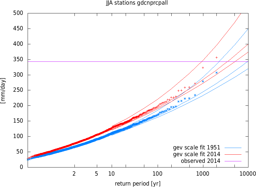
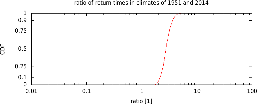
The ratio of return times is often a number that is communicated, so a separate plot is drawn at the end of the page showing the CDF of this ratio derived from a non-parametric bootstrap procedure. TODO: convert this to a FAR distribution. In this case a ratio of one is excluded.
Now that a trend has been detected in the observations, we turn to the theory. Increases in daily precipitation extremes have been found in the data and in climate model output, and are expected on the basis of physics. Temperatures in this part of the world have risen and this rise has been attributed to anthropogenic influences. When I finished writing the paper I will add the quantitative numbers here that conclude the attribution study.